
Part 3 of the “Docker for Data Professionals” Series
Welcome to Part 3! By now, you’ve built your first custom Docker image and containerized a data analysis script. Pretty empowering, right?
But here’s the problem: in Part 2 when you ran docker run my-analysis:v1.0 then stopped that container, everything disappeared. Your output plot? Gone. Any models you trained? Vanished. This is Docker’s “ephemeral” nature.
But wait. If everything disappears, how do data professionals actually use Docker? How do you save your trained models? Work with large datasets? Build complete data stacks with databases and APIs?
You saw a glimpse of that in Part 2 when you ran docker run -v $(pwd)/outputs:/app/outputs my-analysis:v1.0, today we’re going into more detail. By the end of this post, you’ll understand data persistence, manage multi-container applications, and orchestrate an entire data science environment with Docker Compose. Let’s get started!
The Ephemeral Container Problem
Hopefully in Part 2 you had a chance to call docker run my-analysis:v1.0. This should’ve created output.png.
# Run the container
docker run my-analysis:v1.0

# Try to find output.png on your machine
ls output.png
# Result: file not found!What happened? The plot was saved inside the container’s filesystem. When the container stopped, that filesystem disappeared. This is by design. Containers are meant to be disposable, reproducible units.
In reality as a data practitioner, you need to:
- Train models that take hours
- Work with datasets too large to copy into Docker images
- Save experiment results and visualizations
- Share data between multiple containers
- Persist database records across restarts
The solution for handling this ephemeral nature are volumes and bind mounts.
Bind Mounts vs Volumes
Docker offers two primary ways to persist data beyond a container’s lifecycle. Understanding when to use each is crucial for efficient data work.
Bind Mounts Allow Direct Access to Your Files
Bind mounts create a direct link between a specific folder on your host machine and a folder inside the container. It’s like a two-way mirror where both sides see the same files in real-time 🪞.
From Part 2
# Mount your local outputs folder to container's /app/outputs
docker run -v $(pwd)/outputs:/app/outputs my-analysis:v1.0

# Now output.png appears in your local outputs/ folder!The syntax is -v /host/path:/container/path. Your local ./outputs folder is linked to the container’s /app/outputs folder. Same file in both locations.
When Do You Use Bind Mounts?
- During development: edit code locally in your favorite IDE, then run in a Docker container. Changes reflect immediately without needing to rebuild.
- Accessing large datasets already on your machine. Let’s say you have 50GB of training data on
~/datasets/. Mount it into Docker containers instead of copying them into Docker images. - Saving outputs (plots, logs, models) you want immediately. No need to copy files out of containers.
- Quick iteration and debugging. For example, you could inspect log files on your machine while the container is running.
Example: I keep some training data in ~/data/ on my laptop. I mount it read-only to containers: -v ~/data/:/data:ro. The container can read the data but can’t accidentally corrupt it. This gives me peace of mind 😌.
# I keep training data locally and mount it read-only
docker run \
  -v ~/data/imagenet:/data:ro \  # Read-only mount (can't corrupt data)
  -v $(pwd)/models:/models \      # Save trained models locally
  -v $(pwd)/logs:/logs \          # Logs appear on my machine
pytorch-training:v1.0Docker Volumes Manage Storage
Docker volumes are storage locations managed entirely by Docker. You don’t pick the location, Docker does (it’s usually somewhere like /var/lib/docker/volumes/).
# Create a volume
docker volume create model-checkpoints

# Use it in a container
docker run -v model-checkpoints:/models my-training-job:v1.0

# List all volumes
docker volume ls

# Inspect a volume
docker volume inspect ml-checkpoints

# Remove a volume (careful!)
docker volume rm model-checkpointsWhen Do You Use Volumes?
- Database storage (Postgres, MongoDB, Redis, etc.). Their data must persist even after a Docker container restarts.
- During production deployments. Volumes are managed by Docker, making them easier to backup, migrate, and manage at scale.
- When sharing data between containers, multiple containers can mount the same volume. For example, a training container writes models while a serving container reads them.
- Long-lived data that outlasts individual containers.
- Better performance on Mac/Windows (bind mounts can be slower).
- When you don’t need direct file access (like manually editing files), volumes are simpler to use.
Example:
# PostgreSQL with persistent volume
docker run \
  -v postgres-data:/var/lib/postgresql/data \
  -e POSTGRES_PASSWORD=secret \
  postgres:15

# Even if you stop and remove this container, your data is safe in postgres-data volumeHow Docker Tells Them Apart
Both bind mounts and named volumes use the same -v flag in docker run commands, and both appear under the volumes: key within a service definition in docker-compose files. So how does Docker know which one you’re using?
💡 Hint: look at what’s on the left side of the colon.
# Bind Mount - Path on left side (starts with /, ./, ~/, or $(pwd))
docker run -v /home/user/data:/data my-app:v1.0        # Absolute path
docker run -v ./outputs:/app/outputs my-app:v1.0       # Relative path
docker run -v ~/datasets:/data my-app:v1.0             # Home directory
docker run -v $(pwd)/models:/models my-app:v1.0        # Current directory

# Volume - Just a name on left side (no slashes)
docker run -v my-volume:/data my-app:v1.0              # Named volume
docker run -v postgres-data:/var/lib/postgresql/data postgres:15In docker-compose files the same rules apply.
services:
  app:
    volumes:
      # Bind mounts (paths with ./ or /)
      - ./notebooks:/home/jovyan/work     # Bind mount
      - ./data:/home/jovyan/data          # Bind mount
      - /absolute/path:/app/data          # Bind mount

      # Named volumes (just names, no slashes)
      - postgres-data:/var/lib/postgresql/data  # Volume
      - my-models:/models                       # Volume

volumes:
  # Declare named volumes here
  postgres-data:
my-models:If the left side looks like a file path, Docker treats it as a bind mount. If it’s just a name, then it’s a named volume.
Docker will automatically create a named volume if it doesn’t exist. For bind mounts, Docker will create the directory on your host machine if it doesn’t exist.
Quick Comparison
| Feature | Bind Mounts | Volumes |
| Location | You choose | Docker manages |
| Access | Direct file access | Through Docker only |
| Performance | Fast on Linux, slower on Mac/Windows | Optimized everywhere |
| Backup | Your responsibility | Docker tools available |
| Use Case | Development work, datasets | Production, databases |
Port Mapping: Accessing Services in Containers

Ever wondered how that Jupyter notebook from Part 1 was accessible in your browser? That’s thanks to port mapping 🔌.
Containers have their own network. To access services inside them, you need to map container ports to your machine’s ports. Think of it like assigning the container’s port(s) to your machine’s port(s).
# Run Jupyter, map container port 8888 to your port 8888
docker run -p 8888:8888 jupyter/datascience-notebook

# Access at http://localhost:8888The syntax is -p HOST_PORT:CONTAINER_PORT.
# Container's port 5000 → Your machine's port 3000
docker run -p 3000:5000 my-flask-api:v1.0

# Now visit http://localhost:3000Whatever application is available within the container’s port can now be viewed on your machine’s port.
Multiple ports:
docker run \
  -p 8888:8888 \  # Jupyter
  -p 6006:6006 \  # TensorBoard
my-ml-environment:v1.0Common Ports Used for Data Work:
- 8888: Jupyter Lab/Notebook
- 5000: Flask APIs
- 8501: Streamlit apps
- 5432: PostgreSQL
- 6379: Redis
- 6006: TensorBoard
Using Environment Variables
Please tell me you’re not hard-coding database passwords in your code 👀. You should never hardcode secrets in your Dockerfile nor should you commit docker-compose files with real passwords. Always use environment variables or secret management tools in production.
It’s a good thing Docker makes it easy to inject configuration and secrets at runtime with environment variables.
# Pass environment variables
docker run \
  -e DATABASE_URL=postgresql://localhost/mydb \
  -e API_KEY=your-secret-key \
my-app:v1.0In your Python code, you’d write something like the example below to use environment variables that are already defined.
import os

DATABASE_URL = os.getenv("DATABASE_URL")
API_KEY = os.getenv("API_KEY")You can use .env files when working with multiple variables.
Creating an .env File
DATABASE_URL=postgresql://localhost/mydb
API_KEY=your-secret-key
MODEL_PATH=/models/latestCalling a Docker Command with the .env File
docker run --env-file .env my-app:v1.0.env to your .gitignore!
Never commit secrets to version control.
Using Docker Compose 👩🏾🍳
Remember our food analogy? If the Dockerfile is the recipe, a Docker image is the frozen meal, and the Docker container is that meal heated up and served, then Docker Compose is the chef coordinating an entire multi-course meal.
Most data projects need multiple services.
- Jupyter for development
- PostgreSQL for data storage
- Redis for caching
- MLflow for experiment tracking
Starting each manually with docker run gets tedious fast. Docker Compose lets you define everything in one YAML file and start your entire stack with one command.
Building Your First Docker Compose Stack
Let’s build a practical data science environment containing Jupyter, PostgreSQL, and MLflow.
Since the original MLflow Docker image doesn’t include psycopg2, which is needed to connect to PostgreSQL, we’ll need to create a custom Dockerfile for MLflow with psycopg2 installed. The docker-compose.yml will build that custom image for us.
Dockerfile.mlflow
FROM ghcr.io/mlflow/mlflow:latest

RUN pip install psycopg2-binaryWe’ll do the same thing for our Jupyter image. We’ll need to customize it by adding psycopg2 and other missing libraries (using a requirements.txt is a good idea too).
Dockerfile.jupyter
FROM jupyter/datascience-notebook:latest

RUN pip install psycopg2-binary sqlalchemy typing-extensions>=4.6.0 mlflowCreate the docker-compose.yml file
version: '3.8'

services:
  # Jupyter for development
  jupyter:
    build:
      context: .
      dockerfile: Dockerfile.jupyter
    ports:
      - "8888:8888"
    volumes:
      - ./notebooks:/home/jovyan/work
      - ./data:/home/jovyan/data
    environment:
      - JUPYTER_ENABLE_LAB=yes
      - MLFLOW_TRACKING_URI=http://mlflow:5000
    depends_on:
      - mlflow

  # PostgreSQL for data storage
  postgres:
    image: postgres:15
    ports:
      - "5432:5432"
    environment:
      - POSTGRES_DB=ml_data
      - POSTGRES_USER=datauser
      - POSTGRES_PASSWORD=changeme
    volumes:
      - postgres_data:/var/lib/postgresql/data

  # MLflow for experiment tracking
  mlflow:
    build:
      context: .
      dockerfile: Dockerfile.mlflow
    ports:
      - "5008:5000"
    command: mlflow server --host 0.0.0.0 --backend-store-uri postgresql://datauser:changeme@postgres/ml_data
    depends_on:
      - postgres

# Named volumes for persistence
volumes:
postgres_data:Error response from daemon: Ports are not available: exposing port TCP 0.0.0.0:5000 -> 0.0.0.0:0: listen tcp 0.0.0.0:5000: bind: address already in use
It’s okay to change ports; you have a little over 65,000 of them to choose from 😉.
– Mac/Linux:
lsof -i :5000
– Windows:
netstat -ano | findstr :5000
Let’s go through each component of the Docker Compose file.
Services: Each service is a container. They can talk to each other by service name as the hostname. For example, Jupyter can reach MLflow at http://mlflow:5000 (notice how it’s not localhost:5000).
Volumes: ./notebooks:/home/jovyan/work is a bind mount. If you don’t have a folder called notebooks/, Docker will create it for you. Your local notebooks/ folder syncs with the container’s work/ folder. Edit files either in Jupyter or locally and the changes will appear instantly on the other side 🪞.
postgres_data:/var/lib/postgresql/data is a volume. Docker manages this storage. Your database persists even when you run docker-compose down.
test.ipynb, whatever changes I make to one side will reflect on the other side. It’s like an equation (for all my math nerds 🤓)Ports: This is where you map your host ports to the container’s ports. Each service exposes different ports.
Environment: This is where you can pass environment variables or other configurations to each container. In the example docker-compose.yml file we had
environment:
- MLFLOW_TRACKING_URI=http://mlflow:5000This sets an environment variable inside the Jupyter container which we can use.
import mlflow
import os

# Automatically uses MLFLOW_TRACKING_URI from environment
mlflow.set_tracking_uri(os.getenv("MLFLOW_TRACKING_URI"))
mlflow.log_param("learning_rate", 0.01)This is handy since we’re not hard-coding URLs. If we needed to change the MLflow port in docker-compose.yml, then everything would update automatically and the code stays portable.
Depends On: Noticed the depends_on sections within the docker-compose.yml file? This is important for multi-container applications. Services need to start in the right order. If Jupyter starts before MLflow is ready, it can’t connect. If MLflow starts before PostgreSQL is ready, it crashes trying to connect to a non-existent database.
depends_on creates a Directed Acyclic Graph (DAG) which is essentially a dependency chain.
jupyter:
  depends_on:
    - mlflow  # Start MLflow before Jupyter

mlflow:
  depends_on:
- postgres # Start PostgreSQL before MLflowIn the example above, we’re ensuring that PostgreSQL starts first, then MLflow, and finally Jupyter.
depends_on only waits for the container to start, not for the service inside to be ready. PostgreSQL might take 5-10 seconds to fully initialize after the container starts. This is usually fine, but if you see connection errors on first startup, just wait a few seconds and try again. Most production setups use health checks or retry logic to handle this.
Running Your Stack
# Start everything
docker-compose up

# Start in background (detached mode)
docker-compose up -d

# Check what's running
docker-compose ps

# View logs
docker-compose logs jupyter
docker-compose logs -f  # Follow logs

# Stop everything
docker-compose down

# Stop and remove volumes (careful!)
docker-compose down -vYou should now have:
- Jupyter Lab at http://localhost:8888
- PostgreSQL at localhost:5432
- MLflow UI at http://localhost:5008
If you’re in detached mode you can get your Jupyter token by calling:
docker-compose logs jupyter | grep -E "token=|http://127.0.0.1:8888" | tail -5If you’re using attached mode, the logs are printed on the screen, so you could scroll through and find it.
All three services can communicate with each other! Your Jupyter notebooks can connect to PostgreSQL using host='postgres' (not localhost!).
Practical Workflow Example
1. Start the environment
docker-compose up -d2. Develop in Jupyter at http://localhost:8888.
Docker created the ./notebooks folder in my current directory (I didn’t have it before). Within Jupyter Lab there’s a folder called work/, anything that I add to work/ will be copied over to the notebooks folder on my local machine. Changes stay even after I shutdown the containers.
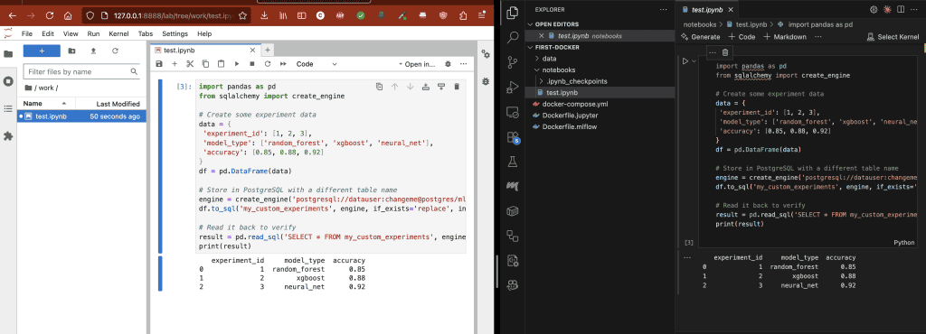
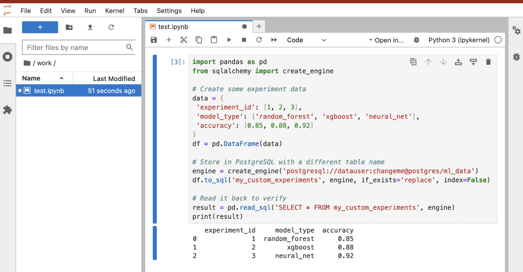
3. Store data in PostgreSQL
import pandas as pd
from sqlalchemy import create_engine

# Create some experiment data
data = {
 'experiment_id': [1, 2, 3],
 'model_type': ['random_forest', 'xgboost', 'neural_net'],
 'accuracy': [0.85, 0.88, 0.92]
}
df = pd.DataFrame(data)

# Store in PostgreSQL with a different table name
engine = create_engine('postgresql://datauser:changeme@postgres/ml_data')
df.to_sql('my_custom_experiments', engine, if_exists='replace', index=False)

# Read it back to verify
result = pd.read_sql('SELECT * FROM my_custom_experiments', engine)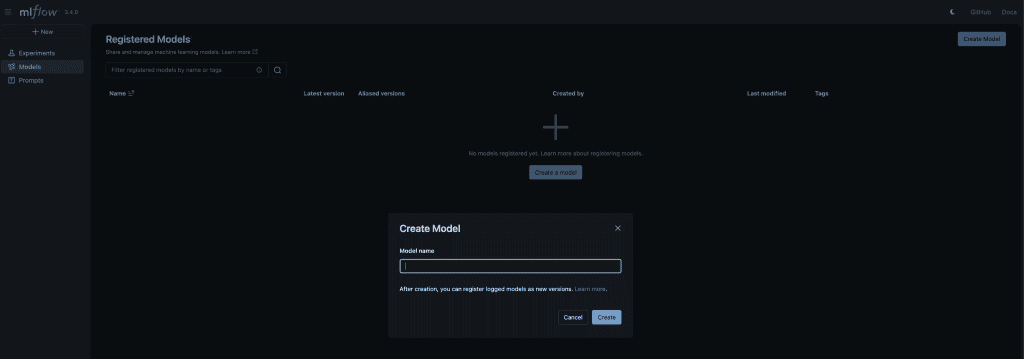
print(result)4. Track experiments with MLflow
import mlflow
import os

# use environment variable or fallback
tracking_uri = os.getenv("MLFLOW_TRACKING_URI", "http://mlflow:5000")
print(f"Connecting to: {tracking_uri}")

mlflow.set_tracking_uri(tracking_uri)

# quick test
print("MLflow version:", mlflow.__version__)
print("Tracking URI:", mlflow.get_tracking_uri())

# creating a test experiment
mlflow.set_experiment("test_experiment")
print("Experiment set successfully!")5. Stop when done
docker-compose down # Database data persists in the volume!The next day I’d run docker-compose up -d and everything is exactly as I left it. No reinstalling, no reconfiguring.
Side Note on the -d Flag
When you run docker-compose up without the -d, your terminal is “attached” to the containers. You see all the logs streaming live, but you can’t use your terminal for anything else. Press Ctrl+C and everything stops.
When you use docker compose up -d, the -d stands for detached mode. Docker Compose starts all your services in the background and gives you your terminal back. The services keep running even if you close the terminal.
-d or no -d?
Attached mode is good for debugging. You see logs immediately and can stop everything with Ctrl+C.
Detached mode is great for normal workflows. Start your stack, get your terminal back, and continue working as usual. When you need to stop the stack you’d run docker-compose down.
Let’s dive into some other features Docker has to offer.
Overriding Different Environments
Skip to Here Are Some Other Tips for Docker Compose 🐳
An awesome feature about Docker Compose is the ability to layer configurations. This lets you have a base setup that works everywhere, then customize it for development, staging, or production without duplicating code.
The problem: You need different settings for different environments:
- Development could need mounts to local code, debug mode enabled, and smaller test databases.
- Production, on the other hand, wouldn’t need local mounts, nor would it need debug mode enabled, and it would use production-grade databases.
You could maintain separate docker-compose.yml files for each environment, but that means duplicating like 90% of the configuration. When you update one, you have to remember to update all the others. Who has time for all that? Not me and neither should you 🤨.
The solution is to override files.
How Overrides Work
Docker Compose automatically looks for these files (in order):
docker-compose.yml(this is the base configuration, it’s always used)docker-compose.override.yml(automatically applied if it exists)
Think of an override like CSS (if you’ve ever developed a website). The base file sets the defaults while the override file changes specific things.
Example Base Configuration (docker-compose.yml)
version: '3.8'

services:
  api:
    image: my-ml-api:latest
    ports:
      - "5000:5000"
    environment:
- LOG_LEVEL=infoDevelopment Override (docker-compose.override.yml)
version: '3.8'

services:
  api:
    # Override: mount local code for live editing
    volumes:
      - ./src:/app/src
    # Override: enable debug mode
    environment:
      - DEBUG=true
      - LOG_LEVEL=debug
    # Add a new port for the debugger
    ports:
- "5678:5678"When you run docker-compose up, Docker automatically merges these two files. Your API service now has:
- The image from the base file
- The port 5000 from the base file
- The mounted volume from the override
- Debug environment variable from the override
- An additional debug port from the override
The magic 🪄: Your teammates can have different override files without affecting each other. Just add docker-compose.override.yml to .gitignore!
Here’s a Data Science Example
Base Config (docker-compose.yml) – This is Committed to Git
version: '3.8'

services:
  jupyter:
    image: custom-jupyter-image:v1.0.0
    ports:
      - "8888:8888"
    volumes:
      - ./notebooks:/home/jovyan/work

  postgres:
    image: postgres:15
    environment:
      - POSTGRES_DB=ml_data
      - POSTGRES_USER=user
- POSTGRES_PASSWORD=changemePersonal Override (docker-compose.override.yml) – NOT Committed in Git
version: '3.8'

services:
  jupyter:
    # Mount your personal dataset
    volumes:
      - /Users/yourname/big-datasets:/data
    # Give Jupyter more memory
    deploy:
      resources:
        limits:
          memory: 8G

  postgres:
    # Use a faster volume driver on your Mac
    volumes:
      - postgres_data:/var/lib/postgresql/data:delegated

volumes:
postgres_data:Now your setup has your personal datasets and memory limits, but your teammate can have completely different overrides without any conflicts!
Production Overrides
For production, you typically use a different override file.
docker-compose.yml with an API Service
version: '3.8'

services:
  api:
    image: python:3.11-slim
    ports:
      - "8000:8000"
    volumes:
      - ./app:/app
    working_dir: /app
    command: python -m http.server 8000
    environment:
      - DEBUG=true
      - LOG_LEVEL=info

  jupyter:
    image: custom-jupyter-image:v1.0.0
    ports:
      - "8888:8888"
    volumes:
      - ./notebooks:/home/jovyan/work

  postgres:
    image: postgres:15
    environment:
      - POSTGRES_DB=ml_data
      - POSTGRES_USER=user
- POSTGRES_PASSWORD=changemedocker-compose.prod.yml
version: '3.8'

services:
  api:
    # Don't mount local code in production!
    volumes: []
    environment:
      - DEBUG=false
      - LOG_LEVEL=warning
    # Production-grade restart policy
restart: alwaysTo use it call
docker-compose -f docker-compose.yml -f docker-compose.prod.yml up -dThe -f flag lets you explicitly specify which files to layer together.
Key Takeaway: Overrides let you keep one source of truth (base file) while customizing for different needs. It’s like having a template that everyone uses, with individual tweaks here and there.
Here Are Some Other Tips for Docker Compose 🐳
Scaling Services
Sometimes you need multiple instances of a service.
# Run 3 Jupyter instances (useful for team environments)
docker-compose up --scale jupyter=3Rebuilding After Code Changes
Use this if you made changes to your Dockerfile or want to rebuild images.
# Rebuild images before starting
docker-compose up --build

# Force rebuild without cache
docker-compose build --no-cacheExecuting Commands in Running Services
This is for when you need to run a one-off command in a running service.
# Open PostgreSQL shell
docker-compose exec postgres psql -U datauser ml_data

# Run a Python script in the notebook service
docker-compose exec jupyter python /home/jovyan/work/process_data.py

# Open a bash shell
docker-compose exec api bashThe Difference Between exec and run:
docker-compose exec: Run command in an already running containerdocker-compose run: Start a new container to run a command
# This starts a NEW container just to run this command
docker-compose run jupyter python my_script.pyCongratulations! You just:
- Understood ephemeral containers vs persistent data
- Mastered volumes and bind mounts
- Mapped ports to access services
- Configured containers with environment variables
- Built a multi-container data science stack with Docker Compose
Homework 📚

Exercise 1: Experiment
Modify the docker-compose.yml to add a Redis service. Use image: redis:7 and map port 6379.
Exercise 2: Practice Persistence
Run your compose stack, create data in PostgreSQL, stop everything with docker-compose down, then start again. Verify your data is still there!
Exercise 3: Project
Think about your current data project. What services would it need? Sketch out a docker-compose.yml for it.
In Part 4 we’ll see examples of ML use cases, GPU support, debugging techniques, and production-ready patterns. We’ll containerize a complete ML model serving API!
Want the quick command reference? Grab the Docker for Data Professionals Cheat Sheet to keep these commands handy!
Remember: Docker Compose isn’t just for production. It’s a massive productivity boost for development. You’re literally running an entire data stack with one command. Happy coding 🚀!