Statistics can be a confusing subject. Firstly, it’s math heavy, and I’m not surprised when someone has gripes about math. Heck, I’m pursuing my master’s in applied mathematics, and I have grievances with it at times 🤷🏾♀️.
But statistics and probabilities are essential for data analysis, data science, and machine learning. To take your analyses to the next level or understand why/how your machine-learning algorithms work, you’ll need to have knowledge of the underlying math. Otherwise, the work that you do could be misleading at best and fraudulent at worst.
A concept that many people have trouble with is the p-value. And I’m not being hyperbolic. Plenty of papers and blog posts have written on how the p-value is an antiquated number that serves more problems than solutions.
More researchers and scientists are adopting a Bayesian approach to their statistical analysis. But in the meantime, the frequentist approach is the methodology most people first learn in high school or college. And it is usually the only school of thought they know. So even though there are a lot of issues with the p-value and hypothesis testing in general, it’s safe to say those methods aren’t going anywhere anytime soon.
That’s fine; it’s still a good idea to better understand how the p-value is used so that when you create your own analyses or look at other people’s work, you’ll have a higher level of scrutiny.
First and foremost, there are two ways to reject the null hypothesis:
- Geometric (looking at the rejection region under the probability density function)
- Numeric (viewing the p-value as a probability)
I’ll write about the rejection region first so the intuition can carry over into how the p-value is used.
Let’s Start with a Toy Example
There’s an anime I’ve been watching called Spy X Family. It’s a very popular show; I think a major reason for its popularity is thanks to Anya and her antics 🤣.

In episode 10, the audience is introduced to a character named Bill Watkins, and Bill is no ordinary 6 year old. The child looks like a grown man and has incredible strength (that’s anime for you), but it had me wondering if his stature is unusual or if it’s the norm.
Yup, I’m using an anime for my toy example, but this is only to conceptualize an idea. In fact, I encourage you to use a topic you enjoy or are passionate about and try to incorporate it into your learning!
Since this is an anime, I will have a couple initial assumptions. One of them is the average height of a 6 year old.
The show is set in some fictional land, but since it’s an anime, I’m going to go with the average height of 6 year old males in Japan. Here’s a link to the table I’m using: https://nbakki.hatenablog.com/entry/Kids_Average_Height_and_Weight_by_Age_in_Japan. We also don’t know Bill’s height, but it’s obvious that he’s abnormally tall for his age, so let’s assume that he’s around 136cm which is about 4’6. (How tall do you think Bill Watkins is? 🤔)


I’ll reference the Jupyter notebook I created at the end of this blog post. For now, I’ll walk through the example.
Null Hypothesis
The average height for a 6 year old male is 116.32 centimeters.
Alternative Hypothesis
The average height for 6 year old males is greater than 116.32 centimeters.
Alpha
We’ll set alpha (our significance level) to be 0.05.
Hypothesis testing is a fundamental statistical test. It’s used when we think the null hypothesis (which is the status quo) doesn’t capture a detail about the population. Like if the accepted belief is that the average height for a 6 year old male is 116.32 centimeters, but we have a sample where the average height is significantly larger.
There could be several reasons our mean sample height differs from the accepted belief. Still, the hypothesis test can only confirm that the null hypothesis is correct (i.e., we fail to reject the null hypothesis) or that the null hypothesis is outdated, and we can pursue our hunch further (i.e., we reject the null hypothesis).
⛔️ Hypothesis testing DOES NOT tell us that our alternative hypothesis is correct. It just gives us the green light to continue investigating why it is the case that our sample statistic is different, which can lead to an updated belief in the underlying population statistic.
⚠️ Notice: If you’re running the code below, you’ll get slightly different results since I’m not using a SEED.
1. Import Statements
Now that we’ve established our null and alternative hypotheses, let’s use Python to aid our analysis.
import numpy as np
import pandas as pd
import matplotlib.pyplot as plt
plt.rcParams["figure.figsize"] = (10,8) # set the figure size for pyplot
import random
from scipy.stats import norm
2. Plot the Probability Density Function
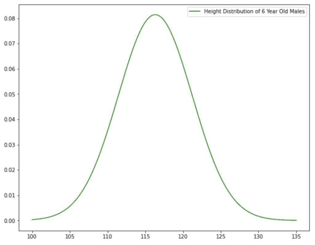
I’ll then plot the height distribution associated with the null hypothesis.
simulated_heights = np.linspace(100, 135, 1000) # heights in centimeters
mean = 116.32 # in cm
std = 4.90 # in cm
pdf_norm = norm.pdf(simulated_heights, mean, std)

plt.plot(simulated_heights, pdf_norm, label="Height Distribution of 6 Year Old Males", color="green")
plt.legend(loc="upper right");
The norm function from scipy.stats can return a probability density function (pdf) using a collection of x values, the mean (µ), and the standard deviation (σ).
simulated_heights is a generated collection of heights 100cm to 135cm; there are 1000 points. 📝 Note: at about 50+ points, the pdf begins to look smooth; anything under 30 points makes the curve look jagged.
The mean and standard deviation are gathered from https://nbakki.hatenablog.com/entry/Kids_Average_Height_and_Weight_by_Age_in_Japan.
3. Create a List of Sample Heights and Add Bill’s Height
# sampling 20 random male students from a class
class_4_heights = np.random.uniform(105, 120, 20)

# I'm adding Bill's height at the end of the list
np.append(class_4_heights, 136.0)
class_4_heights = class_4_heights.round(2)

# print a list of heights from a sample class of 1st graders
print(class_4_heights)
As I’ve mentioned, this is an anime, and I can’t get the heights of all the boys in Bill’s class. Which is why I’m using np.random.uniform(). np.random.uniform() will return a float between the range 105cm to 120cm. I only want 19 students since I’ll add Bill’s height at the end of the list.
4.1 Plot the Rejection Region
sample_mean = np.mean(class_4_heights)

plt.plot(simulated_heights, pdf_norm, label="Height Distribution of 6 Year Old Males", color="green")
plt.axvline(sample_mean, ls="--", label="Sample Mean", color="brown")
limit = norm.ppf(0.975, mean, std)
plt.fill_between(simulated_heights, pdf_norm, 0, alpha=0.2, where=(simulated_heights > limit), label="Rejection Region", color="lime")
plt.legend(loc="upper right");

print(f"Our p-value is {norm.sf(sample_mean, mean, std):.3f} which is > 0.05")
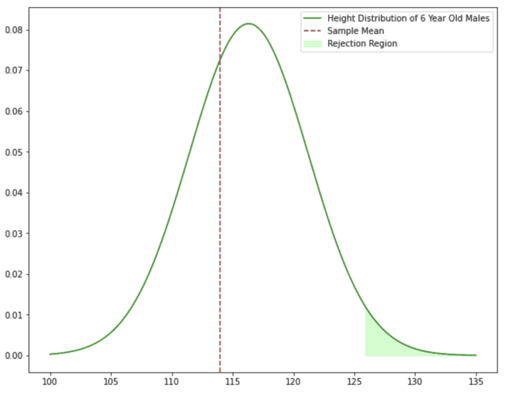
The brown vertical line is the mean of our sample. It’s close to our population mean! Even though Bill was the only outlier, his height didn’t have a notable impact.
The lime-green shaded portion is the rejection region. Which is also known as the Type I error. A Type I error is when we reject the null hypothesis even though it is true. With α = 0.05, we say there’s a 1/20 chance of falsely rejecting the null hypothesis.
If our sample mean fell in the rejection region, that would give us the okay to reject the null hypothesis. But remember that there’s a 1/20 chance that our rejection is wrong. In other words, we would be 95% confident in our judgment call.
Since our sample mean isn’t within the rejection region, we fail to reject the null hypothesis.
4.2 Using the P-Value
There are three ways to interpret the p-value, depending on whether the test is right-tailed, left-tailed, or two-tailed. For the toy example, I'm focusing on the right-tailed test.
For a right-tailed test, the p-value is the probability of getting another random sample statistic (in our case another random sample mean) greater than or equal to our observed value.
The sample mean was about 113.74 cm, so the p-value would give us the probability of having another random sample’s mean greater than or equal to 113.74 cm.
If the p-value is less than or equal to α, that tells us the chances of getting a statistic like the one we observed in our sample is so slim that it’s rare. This pokes holes in the null hypothesis because we shouldn’t see an extreme observation like that popup if the null hypothesis was true. For whatever reason, the null hypothesis isn’t capturing the underlying nature of our population. Signaling that there’s enough evidence for us to reject the null hypothesis.
However, if the p-value is larger than α, this tells us that the chances of observing our sample statistic aren’t uncommon. It was by coincidence that we got a sample statistic that was a little off from the population’s mean. Nothing to ring an alarm about.
The print statement from earlier displayed:

This means there’s a 68.4 % chance of getting a sample mean greater than or equal to 113.74 cm.
There’s nothing statistically significant about our result, and that’s okay!
P-Hacking
What if I didn’t like my result? Deep down, I know that 6 year old boys are much taller than 116 centimeters. So I decided to sample a bunch of 6 year olds whose heights were closer to Bill’s. How would that change my conclusion?
# gathering heights of 20 male students, where everyone is around Bill's height
tall_class_4_heights = np.random.uniform(125, 136, 20)

# I'm adding Bill's height at the end of the list
np.append(tall_class_4_heights, 136.0)
tall_class_4_heights = tall_class_4_heights.round(2)

# print a list of heights from a class of very tall first graders 😅
print(tall_class_4_heights)

#---------------------------------------------------------------------------
tall_sample_mean = np.mean(tall_class_4_heights)

plt.plot(simulated_heights, pdf_norm, label="Height Distribution of 6 Year Old Males", color="green")
plt.axvline(tall_sample_mean, ls="--", label="Sample Mean", color="purple")
limit = norm.ppf(0.95, mean, std)
plt.fill_between(simulated_heights, pdf_norm, 0, alpha=0.2, where=(simulated_heights > limit), label="Rejection Region", color="lime")
plt.legend(loc="upper left");

print(f"Our p-value is {norm.sf(tall_sample_mean, mean, std):.3f} which is <= 0.05")
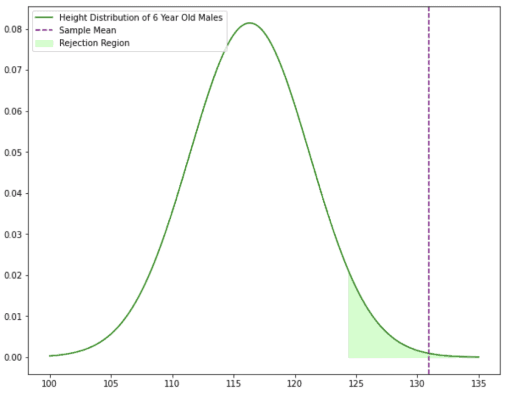
As you can see, my sample mean of ~130.90 cm now falls in the rejection region. So my p-value must be less than or equal to 0.05?!

Sweet! It looks like our p-value is less than alpha which means there’s enough evidence to reject the null hypothesis… Yes and no. This is a blatantly fraudulent example of p-hacking.
P-hacking is when a researcher, analyst, or scientist exploits their EDA to manufacture patterns that would lead to a statistically significant result.
Usually, the researcher will conduct many statistical tests but only report outcomes with significant results. However, excluding certain people from your analysis (in this case: 6 year old males shorter than 125 cm), stopping data collection once you’ve got a result you like, or creating multiple statistical tests from sub-conditions (like looking at heights between 105cm – 110cm, 110cm – 115cm, 115cm – 120cm, 120cm – 125cm, etc. to find significance) are other examples of p-hacking.
Unfortunately, this is fairly common in research/academia. This is why you shouldn’t accept things at face value (even though it is difficult to determine if a researcher has p-hacked their results).
I mentioned that people have issues with the p-value. It’s a number that can range from being confusing to misleading.
Hopefully, this blog post gave you a better understanding of how it’s used and also served as a warning that people can manipulate the p-value to make their analysis look favorable.
As promised here’s the link to my code: https://github.com/cynthiiaa/random-analyses/blob/main/AnimeExample.ipynb
